
Part 1: Well Locations
Last week I wrote a blog post talking about the TX RRC publishing data to the public that previously was only available via a paid subscription.
After downloading the different data sets and examining the various types of data and formats, I decided to take a closer look at the data that might prove to be useful to us and to our Productioneer clients.
It is not uncommon for location and depth data, as well as other well-header and meta data to be incomplete or non-existent during a software migration, after all this data might not be considered crucial for the daily gauge sheets. Especially in the case of Excel gauge sheets, where additional columns are a waste of “prime real estate” and might be considered as cluttering that particular production report.
It would be nice if we have a quick way to pull the Lat Long data in bulk to speed up the on-boarding process.
Where is this data coming from?
The RRC data dump included several Shape Files in the “Digital Map Data” table, I will start by grabbing the well locations from the file called “Well Layers by County” which consists of 255 ArcView Shape Files, one for each county, except one is called wellFED.zip, as in Federal not food, in numbered zip files.

…

Each one of these zip files contains multiple files of different types:
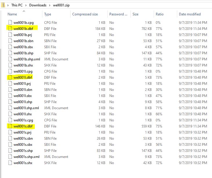
For now, I am only interested in the .DBF files, these are FoxPro dBase files that we will convert into comma separated text files in the next steps. After a quick look at the data in these files, it appears the file ending with …s.dbf is for Surface location, the …b.dbf is for bottom location and we are not sure yet what the …l.dbf is for. They each have a different schema (set of columns)

We will extract the API number and the LAT27 and LON27 columns and use them in a quick Power BI visualization to create the map used for the header of this article. All without trying to write any code, or as we discover later, with as little code as possible.
How: Using Azure Data Lake, Data Factory, Functions and SQL DB to automate the entire process
First, we created a Data Factory pipeline to get the data from the RRC FTP site, load it into the Data Lake, convert the files we need from dbf to csv, then load the csv in a SQL database. The entire pipeline steps look like this. The only place we had to write some code was when we used an Azure Function to convert dbf to csv, more on that step later.

Step 1: Copy RRC files from FTP to Azure Data Lake
This steps grabs all the zipped well shape files on the RRC site, then extracts the contents of each zip file into a separate folder in Azure Data Lake Storage, and it is fast!

This step takes about 1 minute, it reads 255 files and writes 5,832 files.
We only need the .dbf files for now, but I will keep the rest of the files for a later project.
The second step extracts all the .dbf files and puts them in their own folders, this step is optional, just to tidy up.
Data Factory does not have a built-in connector that reads dBase files, so we couldn’t use the default copy activity. My colleague @blake wrote a C# Azure Function that makes use of the DBFDataReader nuget package that he talks about in more details in a separate blog post.
The Function converts all three kinds of files, Surface, Bottom and L files, into CSV files that we then load in the last three steps into a SQL database.
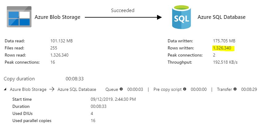
Loading the well locations into SQL was slower, took about 8 minutes to load 1.3 million rows. That is mainly because I have chosen one of the lowest database tiers in Azure since this is not a production environment, to keep the costs low, it would be very easy to scale up with a few clicks and get more speed. The entire project which consists of Data Factory, Storage, Data Lake, Database, Log Analytics and Function App cost $10 so far with an estimated $58 a month total cost at the current low performance tier settings.

Once the well location data was in SQL, I loaded it into the ArcGIS map in Power BI

I also tried the built-in Microsoft map visual and colored the wells by their symbol ID. Note that the built-in map complained about too many objects, and displayed an info message about only showing a representative sampling of the data. That’s ok for the purpose of this exercise…
